Gradient Descent and Backpropagation
Part 3
In the last 2 tutorials, we got introduced to a weird and powerful system called a neural network. We then found out how we can use a process called forward propagation Forward propagation is the process in a neural network where input data moves layer by layer, with each neuron applying its weights, biases, and an activation function. This process produces the network’s final output, which can then be compared to the target for learning. to transform our raw inputs, like the pixels of an image, into a useful output, like “does this image contain a cat?”, based on lots of finely-tuned weights and biases. And, at the end of the last tutorial, I hinted at the way that these networks learn the weights and biases: backpropagation.
3. The Cost Function
Before we delve into how backpropagation works, we first need to understand how we tell neural networks that it's wrong.
This is done through something called the cost function, otherwise known as the loss function. What the cost function does is it compares what the "correct" answer was to what the neural network outputted, and measures how far away the prediction was from that target value. The function assigns a single "error score" number (a scalar A scalar is just a normal number like \(6.1\), \(-\frac{4}{3}\) or \(\sqrt{2}\).) to each set of predictions so that the neural network knows how well it's performing. The higher the cost function, the more wrong the model is.
Now depending on the task of the neural network is, we use different cost functions. For example:
- Mean Absolute Error (MAE) measures the average (mean) difference between the prediction and the target
value. For each datapointIn neural networks, a datapoint is a single input example with
its features and target output, and it forms one part of a larger dataset used for training or evaluation., the
cost function calculates (in pseudo-maths):
\[error = |(correct \text{ } output - predicted \text{ } output)|\]
(the \(|...|\) symbols mean "absolute", and they basically just remove the negative sign if there is one). Then it averages
this result across all the datapoints to get an idea of how wrong the model is overall.
We use MAE when we want to mostly ignore outliers, like when interpreting human-labelled data like product reviews. - Mean Squared Error (MSE) is similar to MAE, except it squares the result at the end,
making it more sensitive to outliers. For each datapoint, error is calculated something like this:
\[error = |(correct \text{ } output - predicted \text{ } output)|^2\]
Then, same as MAE, it takes the average these errors across the entire dataset to provide a sense of overall "wrongness" of the model.
MSE is used a lot in regression tasks, like predicting house prices, where we want to penalise outliers a lot. - Cross Entropy Loss (CE) is another very popular cost function that is used mostly for classification.
In the case where we are trying to do binary classification
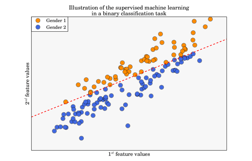
(Kawala, 2015)
Binary classification is a type of machine learning task where the goal is to assign each input to one of two possible "classes". Common examples include spam detection, medical diagnosis (disease vs. no disease), or predicting yes/no outcomes. (an output will fall into 1 of 2 categories), we use the pseudo-formula for one datapoint: \[error = -(correct \text{ } output \cdot \log{(predicted \text{ } output)})+((1-correct \text{ } output) \cdot \log{(1-predicted \text{ } output)})\] or more properly, \[\text{BCE}(y, \hat{y})=-(y\log{(\hat{y})}+(1-y)\log{(1-\hat{y})})\] This formula is slightly more complicated than the previous ones because it uses something called a logarithm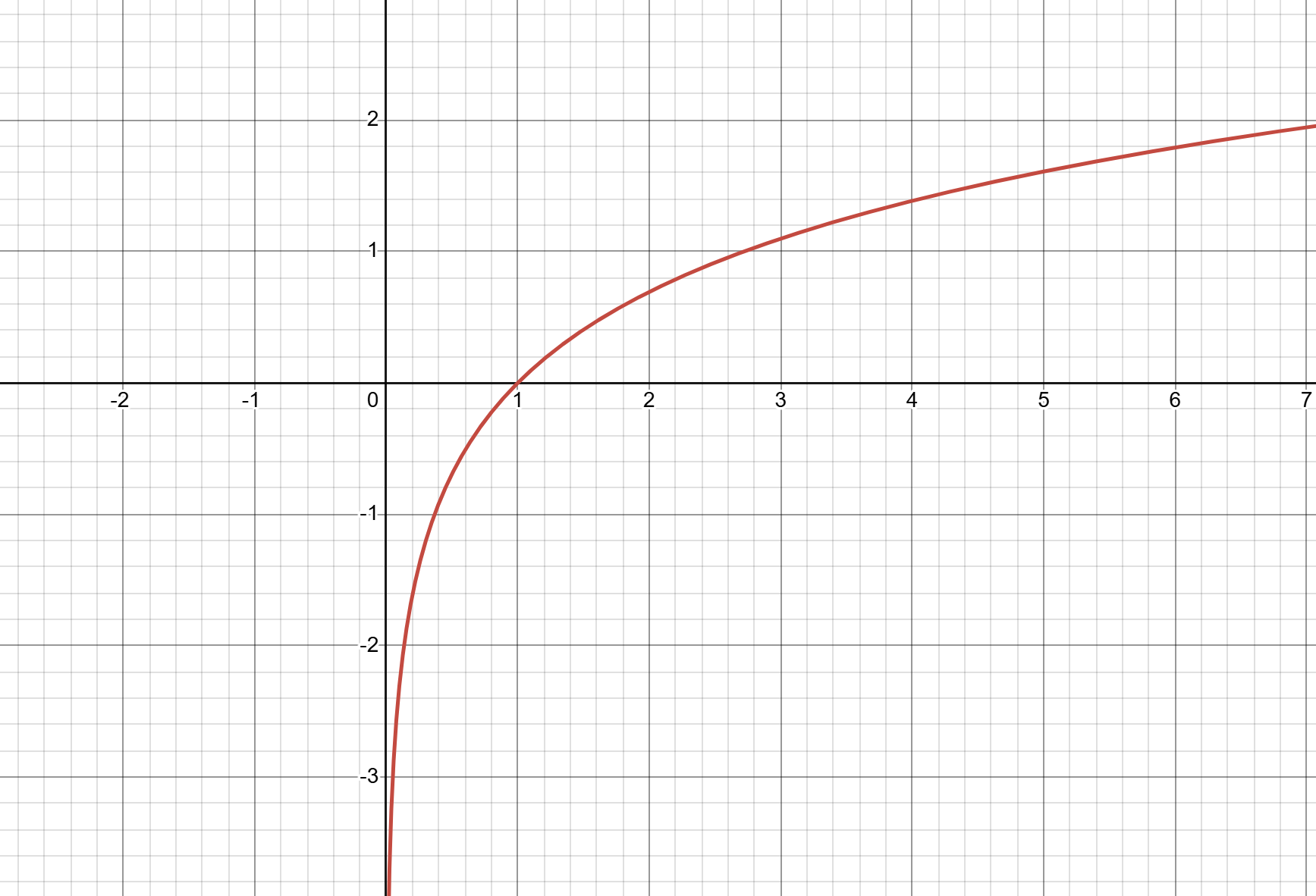
(H.Y. using Desmos)
A logarithm is the inverse of exponentiation, representing the power to which a base must be raised to produce a given number. So: \[a^x=b\] and \[x=\log_a{(b)}\]. This will be explained a bit more in the mathematics section, but what it does is it it penalises confident but wrong predictions much more than less confident ones, which encourages the model to assign high probability to the correct class.
4. Gradient Descent
When we first initialise a neural network that we haven't trained yet, the weights and biases are random, so as you can imagine, the model won't produce very accurate results, so we essentially tell the network, "This is utter trash!", and tell it exactly how far off its predictions were. Once the neural network knows how wrong it is, we use an optimisation algorithm called gradient descent to minimise the "wrongness", which, if you remember, is summarised by the cost function.
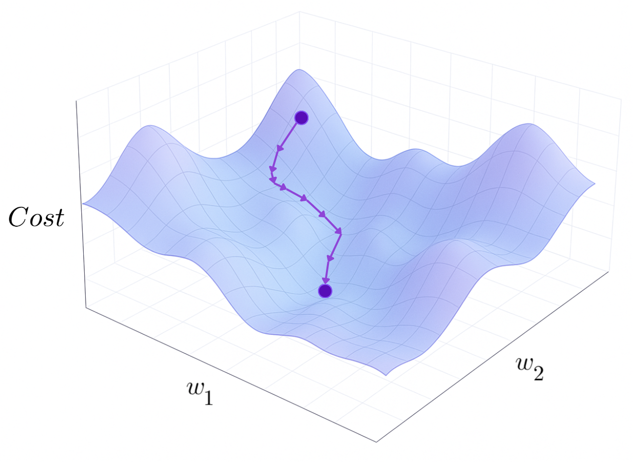
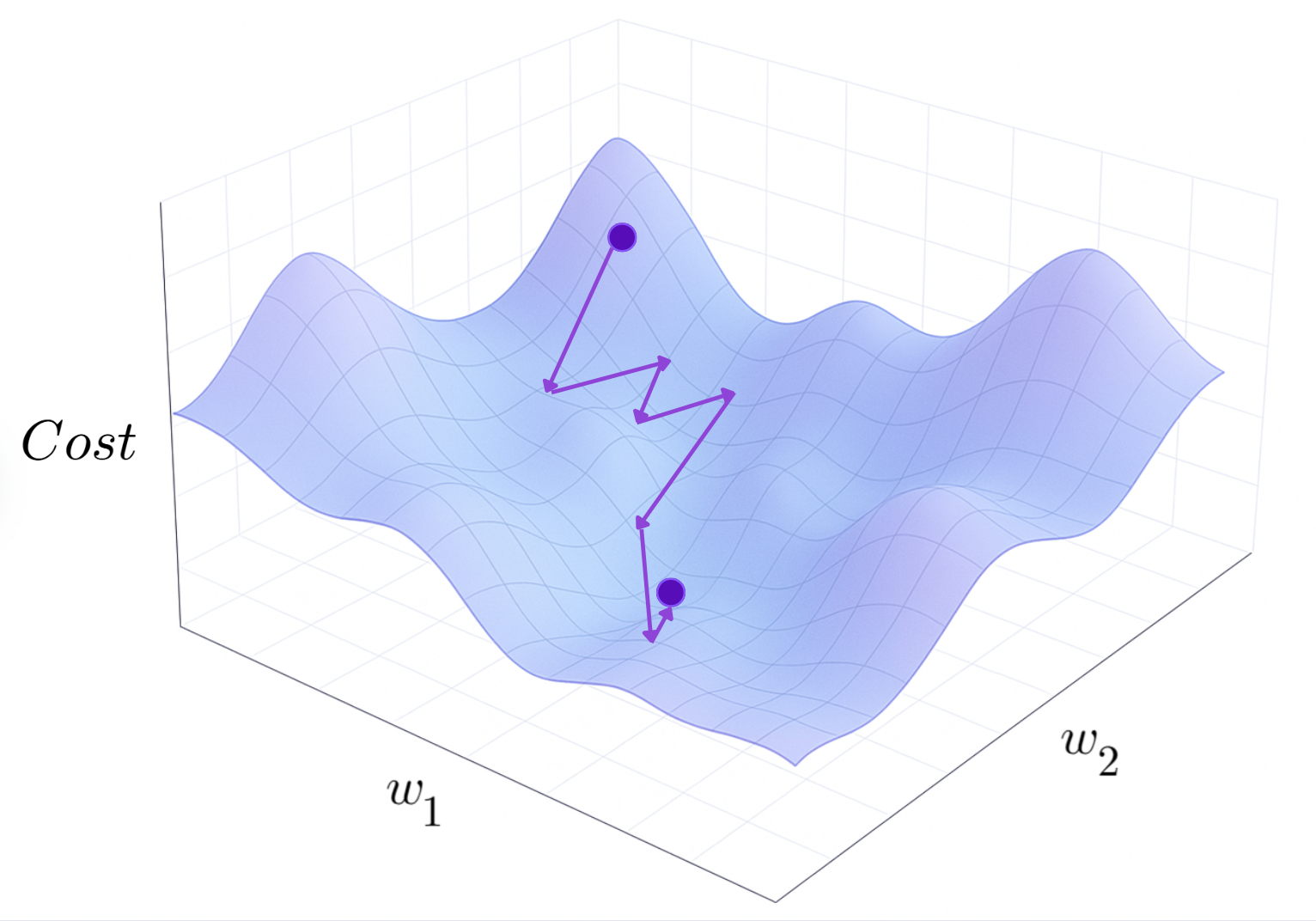
Intuitively, we can think of all the different weights and biases as a ball in high-dimensional space, which is rolling on the surface of the cost function, where the height of the surface is the value of the cost function at with those specific weights and biases:
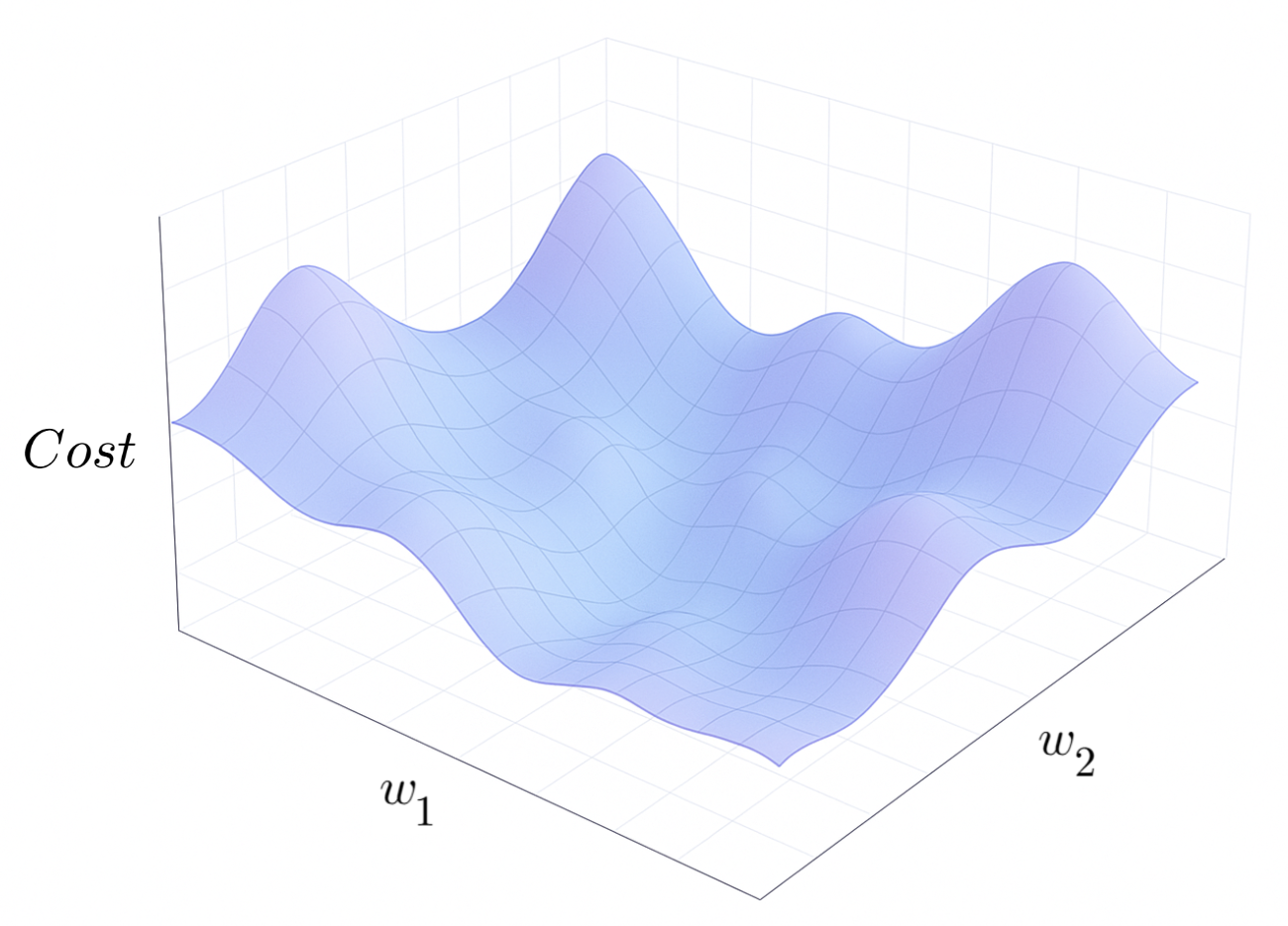
Cost Function Graph (Sora + H.Y. using Canva)
For example, if a neural network had 3 weights and 1 bias, \((-2.0, 2.5, 0.6, -9.3)\), which yielded a cost function value of \(16.1\), then the ball's "position" in space would be \((-2.0, 2.5, 0.6, -9.3,\) \(16.1\)\()\).
What gradient descent does is it iteratively moves the ball (i.e. adjusts the weights and biases) slightly along the cost function surface in the direction of steepest descent.
By taking many small "steps" down the function, the weights and biases will eventually convergeConvergence is the process by which an iterative method, like gradient descent,
approaches a stable solution, meaning a point where further updates no longer cause significant changes because the algorithm is close to a minimum of the cost function. to some local minimum
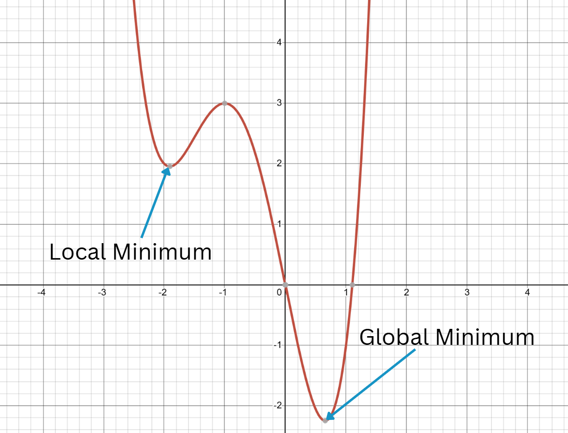
(H.Y. using Desmos)
A local minimum is a point where the function’s value is lower than all nearby points, but not necessarily the lowest overall.
A global minimum is the point where the function achieves its absolute lowest value across the entire domain., where the cost function is very low.
Gradient Descent Diagram (Sora + H.Y. using Canva)
So:
"Gradient descent is the process of iteratively altering the weights and biases in the direction of steepest decrease of the cost function"
5. Backpropagation
However, this all becomes a bit more complicated when we actually want to compute this direction of steepest descent. In a neural network, there are often hundreds or
thousands of nodes across multiple layers all connected in a non-linear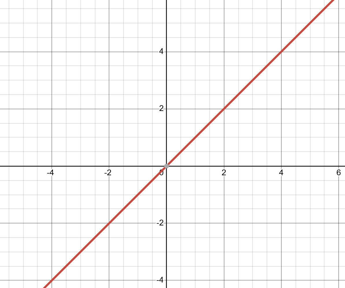
(H.Y. using Desmos)
A linear function, when graphed, produces a straight line. One of the most important features of linear functions is that they always have
the same gradient or "derivative". way. Backwards propagation, backpropagation, or sometimes just
backprop was invented as a way to make this computation easier.
Backpropagation essentially "works backwards", calculating how much each weight and bias contributed to the final outcome. When the neural network is right, then it supports the neurons that contributed to that right answer, and when the model is wrong, backprop figures out which neurons are to blame, and give them less impact on the final result. This is all done using a principle from calculus called the "chain rule" (See the section on mathematics below). If you don't feel like reading about it, it basically says that the impact of neuron A on neuron C is equal to the impact of neuron A on neuron B times the impact of neuron B on neuron C.
See the Mathematics behind Gradient Descent and Backpropagation (Difficulty: ◈◈◈)
Calculus is a big topic and a hard one at that. For that reason, I won't be explaining everything you would typically get taught in a calculus class. I will try to make everything intuitive, but if you don't have a decent mathematical background, bear in mind that you may have to search a few things up and spend some extra time thinking about the content I will teach.
That being said, here's a crash course on the bits of calculus we will need:
Crash Course on Derivatives
Rates of Change and The Derivative
You've probably seen a straight line before, and if you're reading this, there's a good chance you've sketched one too.
Those of you who have taken high-school mathematics may also know what the equation for one is. In 2 dimensions, a straight line
can be graphed using gradient-intercept form \(y=mx+c\), where \(y\) is the height of the graph at the point \(x\), \(m\) is the
gradient, and \(c\) is some constant which is the \(y\)-intercept. In function notation, we can also write \(f(x)=mx+c\).
Something interesting to note here is that the gradient \(m\) doesn't depend on what \(x\) value we have. In other words, the graph has the same
steepness all throughout, so we can represent it by a scalarA scalar is just a normal number like \(6.1\), \(-\frac{4}{3}\)
or \(\sqrt{2}\)., like \(5\) or \(-3\).
However, not all functions are as simple as this.
Take for example the parabola \(f(x)=x^2\).
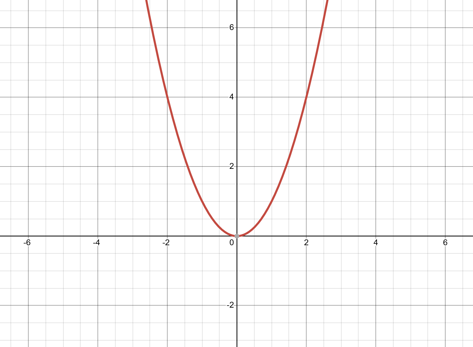 We can clearly see that when \(x\) is negative, the gradient is steeply negative, but as we increase
\(x\), the curve begins to flatten, and when \(x>0\), the steepness of the curve increases to \(+\infty\). This means that, instead of a scalar,
we need a whole function to describe how steep the curve is. For \(f(x)=x^2\), this gradient function is \(f'(x)=2x\). So for example, if
we wanted to calculate the gradient at \(x=3\), we plug \(3\) into the equation to get \(f'(3)=2\cdot3=6\).
We can clearly see that when \(x\) is negative, the gradient is steeply negative, but as we increase
\(x\), the curve begins to flatten, and when \(x>0\), the steepness of the curve increases to \(+\infty\). This means that, instead of a scalar,
we need a whole function to describe how steep the curve is. For \(f(x)=x^2\), this gradient function is \(f'(x)=2x\). So for example, if
we wanted to calculate the gradient at \(x=3\), we plug \(3\) into the equation to get \(f'(3)=2\cdot3=6\).
This concept of a "gradient function" is called the derivative. Every smooth function has a derivative that describes
the rate of change of the function at all points.
There are many different notations that can be used for derivatives, such as Newtonian notation, Lagrangian notation and
Leibniz notation. We will use Leibniz notation in this section because of its great flexibility which we certainly need.
In Leibniz notation, we write derivatives like
\[\frac{d}{dx}\left(f(x)\right)\]
or
\[\frac{df}{dx}\]
These symbols are spoken aloud as "the derivative of the function \(f(x)\) with respect to \(x\)". In plain English, it
basically says: "calculate the gradient function of \(f(x)\) as we change only the variable \(x\)" (of
course we only have 1 variable in this scenario, but if we have more than one variable, we can change what goes on the bottom of the derivative sign)
Derivative Rules
There are a whole lot of rules that tell us exactly how we actually compute these derivatives depending on whats inside the function,
like polynomials, trigonometric functions, logarithms or exponentials. If you plan to learn calculus more formally, you will
need to learn what these rules are, but we're only going to use 4 rules in backpropagation: the sum rule, the constant multiple rule, the power rule and the chain rule.
The sum rule says that if we have a function \(f(x)\) which consists of multiple terms added up, the derivative of \(f(x)\) is the sum of
the derivatives of the individual terms. That's quite a mouthful, so lets write some pseudo-maths to see what this means:
\[\text{the derivative of } (Term \text{ } 1+Term \text{ } 2)\]
\[=(\text{the derivative of }Term \text{ } 1)+(\text{the derivative of }Term \text{ } 2)\]
Using proper notation:
\[\frac{d}{dx}(g(x)+h(x))=\frac{d}{dx}(g(x))+\frac{d}{dx}(h(x))\]
The constant multiple rule says that the derivative of a function \(f(x)\) which consists of some constant multiplied by \(g(x)\) is equal to
that constant multiplied by the derivative of \(g(x)\). In Leibniz notation, we write:
\[\frac{d}{dx}(c \cdot g(x))=c \cdot \frac{d}{dx}(g(x))\]
Also, the derivative of \(x\) is \(1\):
\[\frac{d}{dx}(x)=1\]
The power rule says:
\[\frac{d}{dx}(x^n)=nx^{n-1}\]
where \(n\) is some constant number.
Finally, the chain rule applies to nested functions, and says that if we have a function \(f(u)\) where \(u=g(x)\), the
derivative of \(f(u)\) with respect to \(x\) equals the derivative of \(f\) with respect to \(u\) multiplied by the derivative of \(u\) with respect to \(x\):
\[\text{for some function }f(g(x)) \text{ where } y=f(u) \text{ and } u=g(x),\]
\[\frac{dy}{dx}=\frac{dy}{du} \cdot \frac{du}{dx}\]
Think about the function \(f(x)=\sin{(x^2)}\). Here, we have the outside function \(\sin{(\cdots)}\) and an inside function \(x^2\). To figure out how \(y\)
changes as \(x\) changes, we need to take both layers into account.
Suppose we let
\[y=f(u), u=f(x).\]
We can clearly see that this still equals the original function (just substitute \(u\) in), but now it's made clear that \(y\) depends explicitly on \(u\) and
\(u\) depends explicitly on \(x\). The chain rule says that the entire derivative of \(\sin{(x^2)}\) equals the derivative of \(\sin{(\cdots)}\) times
the derivative of \(x^2\):
\[\frac{d}{dx}(\sin{(x^2)})=\frac{d}{du}(\sin{(u)})\cdot\frac{d}{dx}(x^2)\]
Conveniently, this looks almost like fractions multiplying together. Even though \(\frac{dy}{du}\) and \(\frac{du}{dx}\) are not actual fractions, the notation
is designed so that the \(du\)'s cancel out nicely in your head.
Its okay if you still don't fully get this. You will however need to know this for the upcoming maths, so here are a few good explanations of it:
•Khan Academy Article →
•Calc Workshop Tutorial →
•Professor Dave Explains Video →
(Note: Some of these tutorials use the Lagrangian notation \(f'(x)\). The \('\) means "derivative with respect to whatever variable makes sense in that context".
This is why I said that Leibniz notation is more flexible: we can explicitly define which variable we are taking the derivative with respect to.)
Also, for those of you who want an overview of some other rules not discussed here, I made a resource a few years back that might help you. (There are also heaps of
great YouTube videos out there, like 3Blue1Brown's course on calculus
and the videos made by Professor Dave Explains)
DOWNLOAD RESOURCE ↓
Vector Functions and The Partial Derivative
This is all nice and works well if we only have one variable in the equation, like:
\[f(x)=3x^2\cdot\sin{\left(\frac{2\cos{(x)}}{5\log_2{\sqrt{x+1}}}\right)}+e^{7x-12}\]
But what happens if we have a function that takes in more than one variable? For example, Netwon's law of universal gravitation
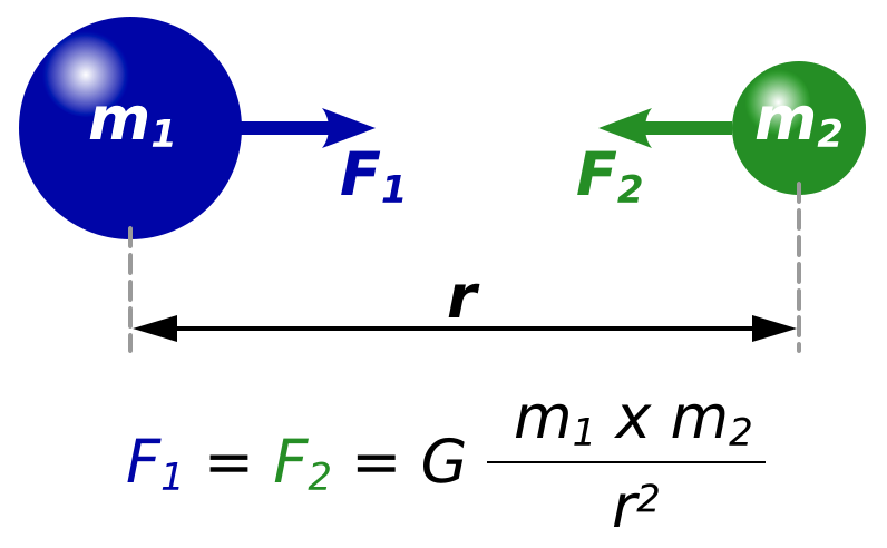
(Wikipedia, 2008)
Newton’s law of gravity says that anything with mass pulls on everything else with a force. The
bigger the masses are and the closer they are, the stronger that pull is. This is described by the equation: \[F_1=F_2=G\frac{m_1 \cdot m_2}{r^2}\] takes in 3 variables:
\[F(m_1,m_2,r)=G\frac{m_1 \cdot m_2}{r^2}\]
where \(G\) is the gravitational constant \(\approx 6.6743 \cdot 10^{-11} m^3kg^{-1}s^-2\).
Here, we have a choice of which variable we want to take the derivative with respect to: \(m_1\), \(m_2\) or \(r\). If we chose, say, \(m_1\), then we will treat all other variables (in
this case \(m_2\) and \(r\)) as a constant like \(G\), \(5.2\) or \(sqrt{3}\). This makes sense because as we change \(m_1\), neither \(m_2\) nor \(r\) change. Another thing thats used just
as a piece of notation with these partial derivatives is that instead of writing \(\frac{d}{dx}\), we write \(\frac{\partial}{\partial x}\) So:
\[\frac{\partial F}{\partial m_1}=G\frac{m_2}{r^2}\]
Why? Because in the equation, we have our variable \(m_1\) multiplied by these assortment of constants, which you may like to group together as \(C\):
\[\text{if }C=G\frac{m_2}{r^2}, \text{ then } F=C \cdot m_1\]
Since we know that \(\frac{d}{dm_1}(m_1)=1\), the constant multiple rule tells us that \(C\), or \(G\frac{m_2}{r^2}\) is our partial derivative.
If you've been sitting here for the past half hour trying to make sense of these abstract symbols, I do recommend you stand up, make yourself a cup of tea, and maybe go for a walk.
This is complicated stuff that you only learn in a second-year university calculus course. Know that you're not alone in being baffled.
If you're ready to continue, please hang on just a little longer. We're almost done with the complicated maths.
Now one thing we can do with these multivariable functionsA multivariable function is a function that depends on two or more independent variables.
Instead of outputting a single value based on one input, it produces a value based on several inputs at the same time. that we couldn't do with single-variable functions is compute
derivatives with respect to multiple variables simultaneously. Intuitively, we think of a multivariable function as some hyper-surface in any number of dimensions (There's 1 dimension for
every input, plus 1 extra dimension for the output):
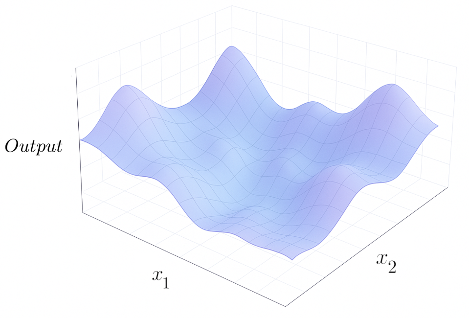 Then our new "gradient function" is a vector sitting on this surface. And the direction it points in is very important: it's the direction of steepest ascent.
Using an analogy, imagine
that you're on some terrain (the multivariable function surface), trying to summit a mountain (let's call it Mount Thill). This new "gradient function" takes in as its input you're location, and
outputs (as a vector), which direction will get you up Mount Thill the quickest (there are some magnificent views up the top).
Symbolically, we write:
\[\nabla f(x_1, x_2, x_3, \cdots, x_n)=\left(\frac{\partial f}{\partial x_1}, \frac{\partial f}{\partial x_2}, \frac{\partial f}{\partial x_3}, \cdots, \frac{\partial f}{\partial x_n}\right)\]
The new symbol \(\nabla\) is called a "nabla" or "del", and its basically our new symbol for derivative when we're talking about this multi-variable gradient function. In the equation, we've defined
the gradient function \(f\) to take in any number of inputs \(x_1\) through \(x_n\), and output a vector that points in the direction of steepest ascent.
Now the last thing you need to know is that the direction of steepest descent is equal to the negative vector pointing in the direction of steepest descent. In pseudo-maths:
\[\text{direction of steepest descent}=-\left(\frac{\partial f}{\partial x_1}, \frac{\partial f}{\partial x_2}, \frac{\partial f}{\partial x_3}, \cdots, \frac{\partial f}{\partial x_n}\right)\]
If you've made it this far, congratulations. Give yourself a pat on the back. You've (basically) learnt 3 years worth of calculus in (hopefully) under an hour. If you're still unsure about any of
this, feel free to contact me or look at some other internet resources. Some good ones include:
•Khan Academy Article (Vector Functions) →
•Khan Academy Article (Intro to Partial Derivatives)→
•Dr. Trefor Bazett Video (The Gradient Vector) →
The Mathematics of Gradient Descent
Alright, so we know that at any point on an \(n\)-dimensional surface, we can find the direction of steepest descent with the equation: \[\nabla f(x_1, x_2, x_3, \cdots, x_n)=-\left(\frac{\partial f}{\partial x_1}, \frac{\partial f}{\partial x_2}, \frac{\partial f}{\partial x_3}, \cdots, \frac{\partial f}{\partial x_n}\right)\] This can actually be used to our cost function to adjust the weights and biases slightly in order to decrease the cost function. Let's start with the biases, because they are a bit easier to deal with since they're vectors. Symbolically for 1 layer, we can write: \[b^{(l)} \leftarrow b^{(l)}-\eta\left(\nabla_{b^{(l)}} C\right)\]
- Calculate the direction of steepest ascent of the cost function \(C\) with respect to the biases \(b^{(l)}\) of layer \((l)\). This is represented as \(\nabla_{b^{(l)}} C\).
- Multiply this vector by the learning rate \(\eta\) (eta). This controls "how big the step is down the mountain".
- Subtract this from the original biases vector to "step down the mountain".
- Update the biases accordingly.
Where \(\eta\) (eta) is the learning rate (the "size of the step we take").
Expanding \(\nabla_{b^{(l)}} C\), we can also write:
\[b^{(l)} \leftarrow b^{(l)}-\eta\begin{pmatrix}\frac{\partial C}{\partial b_1^{(l)}} \\ \frac{\partial C}{\partial b_2^{(l)}} \\ \vdots \\ \frac{\partial C}{\partial b_n^{(l)}}\end{pmatrix}\]
If you read the last section of the derivatives crash course, this looks very similar to \(-\left(\frac{\partial f}{\partial x_1}, \frac{\partial f}{\partial x_2}, \frac{\partial f}{\partial x_3}, \cdots, \frac{\partial f}{\partial x_n}\right)\).
This is because it is! The only difference is that we're taking the partial derivative with respect to the biases of layer \(l\), which we like to represent with a column vector rather than
a row vector. So all this expresion is really saying is:
"Take a step down the cost function in the direction of steepest descent"
And, as we know, a lower cost function means less error, so this is how neural networks learn what the biases should be!
▬▬▬▬▬▬
We can do this same process and use the same equations for our weights too, with a slight change. The biases were vectors, but as we learned last tutorial, weights are put in a matrix
\[W^{(l)} = \begin{bmatrix}
w_{11}^{(l)} & w_{12}^{(l)} & w_{13}^{(l)} & \cdots & w_{1n}^{(l)}\\
w_{21}^{(l)} & w_{22}^{(l)} & w_{23}^{(l)} & \cdots & w_{2n}^{(l)}\\
\vdots & \vdots & \vdots & \ddots & \vdots \\
w_{m1}^{(l)} & w_{m2}^{(l)} & w_{m3}^{(l)} & \cdots & w_{mn}^{(l)}
\end{bmatrix}\]
A matrix is a rectangular grid of numbers or variables. In the context of neural networks, we usually talk about 2D matrices that represent
all the weights (and sometimes biases) between two layers. These matrices normally have \(m \times n\) shape where \(n\) is the input index and the
number of columns, and \(m\) is the output index and the number of rows..
What this means is that our direction of steepest descent is going to be a 2D matrix as well. This might seem counter-intuitive, because the direction of steepest descent (a direction) only required 1 vector for the biases, so why should it require multiple vectors (bundled together in a matrix) for weights? Well, intuitively, we can think of "unpacking" our matrix like this:
\[\begin{bmatrix} \textcolor{blue}{\frac{\partial C}{\partial w^{(l)}_{11}}} & \textcolor{blue}{\frac{\partial C}{\partial w^{(l)}_{12}}} & \textcolor{blue}{\cdots} & \textcolor{blue}{\frac{\partial C}{\partial w^{(l)}_{1n}}} \\ \textcolor{green}{\frac{\partial C}{\partial w^{(l)}_{21}}} & \textcolor{green}{\frac{\partial C}{\partial w^{(l)}_{22}}} & \textcolor{green}{\cdots} & \textcolor{green}{\frac{\partial C}{\partial w^{(l)}_{2n}}} \\ \vdots & \vdots & \ddots & \vdots \\ \textcolor{red}{\frac{\partial C}{\partial w^{(l)}_{m1}}} & \textcolor{red}{\frac{\partial C}{\partial w^{(l)}_{m2}}} & \textcolor{red}{\cdots} & \textcolor{red}{\frac{\partial C}{\partial w^{(l)}_{mn}}} \end{bmatrix}=\begin{pmatrix}\textcolor{blue}{\frac{\partial C}{\partial w_{11}^{(l)}}} \\ \textcolor{blue}{\frac{\partial C}{\partial w_{12}^{(l)}}} \\ \textcolor{blue}{\vdots} \\ \textcolor{blue}{\frac{\partial C}{\partial w_{1n}^{(l)}}} \\ \textcolor{green}{\frac{\partial C}{\partial w_{21}^{(l)}}} \\ \textcolor{green}{\frac{\partial C}{\partial w_{22}^{(l)}}} \\ \textcolor{green}{\vdots} \\ \textcolor{green}{\frac{\partial C}{\partial w_{2n}^{(l)}}} \\ \vdots \\ \vdots \\ \textcolor{red}{\frac{\partial C}{\partial w_{m1}^{(l)}}} \\ \textcolor{red}{\frac{\partial C}{\partial w_{m2}^{(l)}}} \\ \textcolor{red}{\vdots} \\ \textcolor{red}{\frac{\partial C}{\partial w_{mn}^{(l)}}}\end{pmatrix}\] Now that our data is in the "shape" of a vector, we can treat it like a vector direction, and do the same thing we did for the biases. However, we still like to use the matrix version in the notation: \[W^{(l)} \leftarrow W^{(l)}-\eta\left(\begin{bmatrix} \frac{\partial C}{\partial w^{(l)}_{11}} & \frac{\partial C}{\partial w^{(l)}_{12}} & \cdots & \frac{\partial C}{\partial w^{(l)}_{1n}} \\ \frac{\partial C}{\partial w^{(l)}_{21}} & \frac{\partial C}{\partial w^{(l)}_{22}} & \cdots & \frac{\partial C}{\partial w^{(l)}_{2n}} \\ \vdots & \vdots & \ddots & \vdots \\ \frac{\partial C}{\partial w^{(l)}_{m1}} & \frac{\partial C}{\partial w^{(l)}_{m2}} & \cdots & \frac{\partial C}{\partial w^{(l)}_{mn}} \end{bmatrix}\right)\]▬▬▬▬▬▬
Now these two equations for the weights and biases are really all we need to update and adjust these parameters to minimise the cost function. These two equations can be summarised in the single short equation,
\[\theta \leftarrow \theta - \eta \nabla C(\theta)\]
where \(\theta\) represents all our parameters (the weights and the biases).
The fact that such a conceptually deep idea can be summarised and described by just a few symbols is the reason that we use maths in neural networks. Although its hard to learn it, it makes writing down really
complex stuff like this very succinctly.
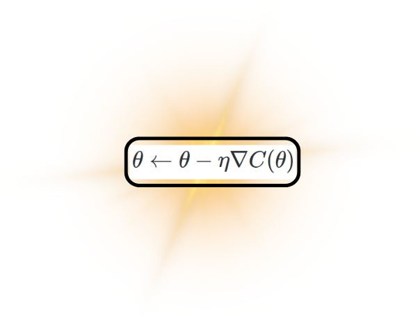
Gradient Descent Formula (H.Y. using Canva + Overleaf)
▬▬▬▬▬▬
Backpropagation
We now only really have 1 problem left: How do we actually compute these partial derivatives? How do we know what \(\frac{\partial C}{\partial w_{32}^{(2)}}\) is? This is the purpose of backpropagation, and its basically "working backwards" from the output all the way to the singular parameter whose effect on the cost function we want to know.
As you may recall, in the previous tutorial about feedforward neural networks (FNNs), we learnt about the process called
forward propagation, which is the process by which we are able to process our inputs through many layers of weights and biases to get to some useful output.
Backwards propagation does the opposite:
"Backpropagation is the process of working backwards from the output to a specific weight or bias to see its effect on the final cost function"
The clever thing that backpropagation does is it uses the chain rule from calculus. As you would recall, the chain rule says that for a composite function \(f(g(x))\): \[\frac{dy}{dx}=\frac{dy}{du}\cdot\frac{du}{dx}\] where \(y=f(u)\) and \(u=g(x)\). This can be applied to partial deriatives as well: \[\frac{\partial y}{\partial x}=\frac{\partial y}{\partial u}\cdot\frac{\partial u}{\partial x}\] And, as the keen reader may notice, if we replace \(f\) with our cost function \(C\) and the independent variable \(x\) with \(w_{ji}^{(l)}\), we now have a better way to compute our partial derivative gradients. After all, we know that the cost function is based on the output, which itself is a composite function of all the different weighted sums. To find how a singular weight or bias affects the final cost function, its helpful to use a tree diagram like this one:
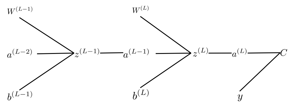
Backpropagation Tree Diagram (H.Y. using Canva + Overleaf)
Here, each function on the left affects the ones on the right, so we can clearly see that the function composition with respect to \(W^{(L-1)}\) say, is \(W^{(L-1)} \leftarrow z^{(L-1)} \leftarrow a^{(L-1)} \leftarrow z^{(L)} \leftarrow a^{(L)} \leftarrow C\). So, combining this knowledge with the chain rule, we can see that \[\frac{\partial C}{\partial W^{(L-1)}}=\frac{\partial C}{\partial a^{(L)}}\cdot\frac{\partial a^{(L)}}{\partial z^{(L)}}\cdot\frac{\partial z^{(L)}}{\partial a^{(L-1)}}\cdot\frac{\partial a^{(L-1)}}{\partial z^{(L-1)}} \cdot\frac{\partial z^{(L-1)}}{\partial W^{(L-1)}}\] Each of these derivatives are pretty easy to compute, then we just multiply them all together to get our final gradient!
▬▬▬▬▬▬
And we're done! (almost) This is how neural networks learn! We use gradient descent, summarised by the formula \(\theta \leftarrow \theta - \eta \nabla C(\theta)\) to figure out how to most quickly minimise our cost function,
and the actual way we compute this is by using the backpropagation and the chain rule from calculus. It's been a bumpy ride, but I hope you've enjoyed it and gotten something out of it. Give yourself a pat on the back, buy yourself an ice-cream. You really do deserve it. Well done.
6. Algorithms for Gradient Descent
Now what we currently have implemented in our neural network is something called batch gradient descent. Batch gradient descent computes the gradient of the cost function using the entire training dataset before updating the parameters. This means every update step takes into account all examples, giving a very accurate estimate of the true gradient direction. While this significantly increases the likelihood of convergence, batch gradient descent is usually computationally expensive with large datasets as each update must take into account all of the training points. Also, batch gradient descent often leads to the parameters getting "trapped" in local minima or saddle points without the "noise" introduced by randomisation.
An alternative to batch gradient descent is something called stochastic gradient descent (SGD). Stochastic gradient descent updates the parameters using just one randomly chosen training example at a time. This is very fast to update and introduces randomness into the optimisation, enabling the algorithm to escape local minima and explore deeper into the cost surface. But because the gradient is based on a single example, updates can become noisy and the cost function may significantly fluctuate rather than gradually decreasing, requiring a careful choice of learning rate and decay strategies.
Stochastic Gradient Descent Diagram (Sora + H.Y. using Canva)
However, most modern neural networks with large datasets (and usually ones more complicated than basic FNNs (More will be discussed in the next tutorial)) use something in between called Mini-batch gradient descent. Mini-batch gradient descent computes the gradient from a random small subset (mini-batch) of training cases, usually 32–512 cases at once. This balances computational efficiency with stable convergence since the mini-batch average gradient is less noisy than SGD but faster to compute than from the whole batch. Mini-batch updates also let us use new technology with multiple "threadsA thread is a small unit of a program that handles one task, while other threads can handle different tasks at the same time. They all share the same memory, so it’s quicker and lighter than running separate programs." (like GPUs), so this is the most widely used version of gradient descent in deep learning.