Feedforward Neural Networks
Part 2
As we've seen, neural networks consist of layers of connected nodesA node in a neural network is a small processing unit that takes input values, performs a simple calculation, and produces an output that helps the network make decisions or predictions. that can identify patterns in data, transforming raw input to useful outputs. What makes them so powerful is that neural networks adapt with time, modifying their configurations until they can recognise images, understand language, or predict the next word in a sentence. But before today's complicated systems existed, the simplest embodiment of this idea was something much simpler: the perceptron.
1. The Perceptron
Frank Rosenblatt
(Wikipedia, 2025)
Frank Rosenblatt (July 11, 1928 – July 11, 1971) was an American psychologist and computer
scientist notable for his work in machine learning and neural networks. introduced the perceptron in 1958,
with the goal of inventing a machine that could learn to recognise patterns from data rather than relying on fixed
instructions. At its heart, the fundamental perceptron is quite simple: it takes in some inputs
For neural networks, the input is the data that is put into the network that is processed to determine an output.,
weightsA weight is a number that determines how much influence a particular input
has on the perceptron’s output. them, adds them together, and passes them through some "activation
An activation function is a rule that decides the perceptron’s output based on the weighted sum of its
inputs." function to produce a binary (\(0\) or \(1\)) output. (Rosenblatt used a certain type of activation function
called a thresholdA threshold function is a function that outputs only 0 up until a
certain "threshold", after which the function will output some non-zero value. function)
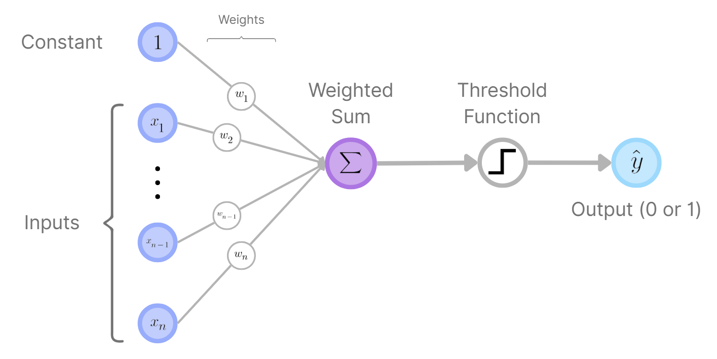
Perceptron Diagram (H.Y. using Canva)
What made it so interesting at the time is that it could adjust its own weights based on errors it made, allowing it to gradually
improve how to classify inputs into one of two outputs. While the perceptron had limitations (it could not solve problems that weren’t
linearly separable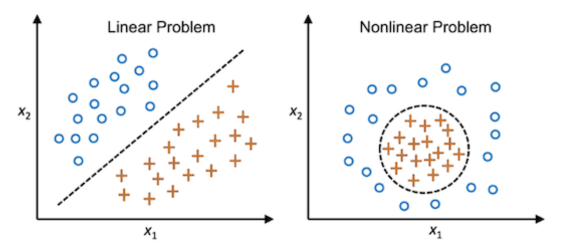
(cmdlinetips, 2021)
A dataset is linearly separable if you can draw a straight line (or flat surface in higher dimensions) that separates the different groups
without overlap., like the XOR problem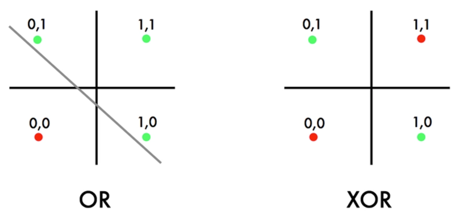
(Jayesh Bapu Ahire, 2020)
The XOR problem is an important problem in machine learning, and involves creating a model that can
correctly output \(1\) when two binary inputs are different (one is \(0\) and the other is \(1\)), and \(0\) when the inputs are the same
(both \(0\) or both \(1\)).), it inspired more advanced models such as multilayer perceptrons, which overcame these
challenges by adding hidden layers.
See the Mathematics behind Perceptrons (Difficulty: ◈◇◇)
Mathematically, a perceptron works by taking many inputs as a vectorIn school, you typically
get taught that a vector is a thing with both a magnitude and a direction. However, in the context of neural networks and computer science
in general, it's more helpful to just think of a vector as a long (or short) list of numbers. \(( x_1, x_2, …, x_{n-1}, x_n)\) and multiplying each value by a corresponding
weightA weight is a number that determines how much influence a particular input has
on the perceptron’s output. \(w\) from \((w_1, w_2, \cdots, w_{n-1}, w_n)\). These results are added with a
bias termA bias is an extra number added to the weighted sum of inputs that allows
the perceptron to shift its decision boundary. \(b\), which produces a weighted sum: \(z = w_1x_1 + w_2 x_2 + \cdots + w_n x_n + b\).
This value \(z\) then goes through an activation function An activation function is a rule
that decides the perceptron’s output based on the weighted sum of its inputs.. In Rosenblatt's design, the perceptron used a simple
step function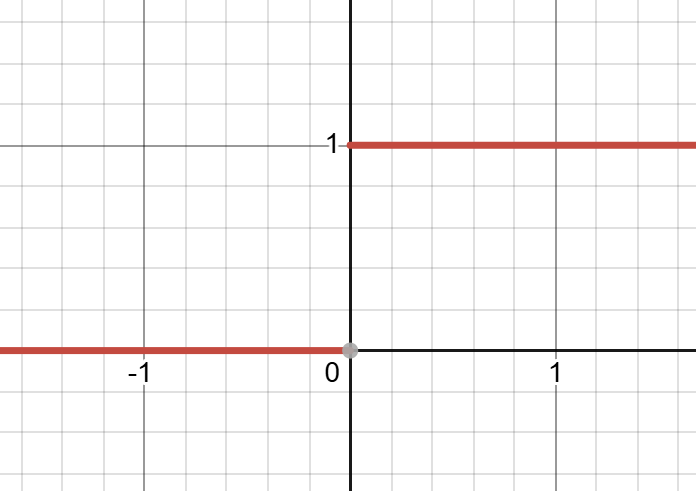
(H.Y. using Desmos)
Step functions are piecewise functions made up of sections of horizontal lines. A common variation of the step function
equals \(0\) up until \(x=0\), after which the function equals \(1\): if \(z > 0\), the perceptron gives \(1\) as its output.
If not, it returns \(0\), therefore dividing the input spaceThe input space is the set of all
possible values that the perceptron’s inputs can take, often visualised as a coordinate system where each axis represents one input.
into 2 distinct regions separated by a straight line (or plane).
Perceptrons are valuable because of how they learn these weights and the bias. When a perceptron makes an incorrect prediction, the weights are changed slightly using the rule:
\[w_i \leftarrow w_i + \eta(y-\hat{y}) x_i\]
- Look at the perceptron’s prediction (\(\hat{y}\)) and compare it to the correct answer (\(y\)).
- Find the difference between the correct answer and the prediction (\(y-\hat{y}\)). This tells you how wrong the perceptron was.
- Multiply that difference by the input value (\(x_i\)) for this particular weight. This figures out how much this input contributed to the error.
- Multiply by the learning rate (\(\eta\)), a small number that controls how big the adjustment should be.
- Add this adjustment to the current weight (\(w_i\)) to get the new weight.
In this formula, \(y\) is the actual output, \(\hat{y}\) is what the perceptron guessed, and the Greek letter \(\eta\) (eta) is the learning rate. This rate is a constant that controls how large the change should be. This rule slowly moves the decision boundary until the perceptron properly divides the training data, assuming the problem can be separated by a straight line. This concept is quite simple, but it is the basis for how neural networks adjust when training, even now.
If this doesn't make sense to you right now, don't worry. In the next tutorial we will look more intuitively and deeply into how this concept of self-learning works. In the meantime, just know that for 1 perceptron, its pretty easy to make it "learn", and that there exists a formula that dictates this.
2. Multilayer Perceptrons
However, a single perceptron is not very useful, as it only works well on linearly separable data
(cmdlinetips, 2021)
A dataset is linearly separable if you can draw a straight line (or flat surface in higher dimensions) that separates the different groups
without overlap.. Most real-world problems are not so simple, like handwriting recognition, for example, where the shapes of letters
overlap in complex ways, or image classification, where categories blur into each other.
To solve these problems, we can use a whole network of these single perceptrons, which we call a feedforward neural network (FNN) or a multilayer perceptron (MLP). FNNs and MLPs connects many perceptrons together in multiple layers, which allow the network to learn far more complex patterns, because instead of a line, decision boundaries can now be curved, segmented, or abstract.

Zoomed-In Neural Network Diagram (H.Y. using Canva)
A simple FNN includes:
- An input layer where raw data arrives (pixels of an image, numbers in a dataset, etc.)
- Hidden layers that find patterns in the data
- The output layer produces the final prediction (e.g., "this is a cat" or "this is a dog")
In this setup, our inputs for each individual perceptron node are simply the values of the perceptrons in the previous layer, as seen in the diagram above. Once it has performed the summation and applied the activation function, the node then displays its result for the next layer of neurons.
Eventually, each perceptron in a layer connects to perceptrons in the next, producing a dense set of weighted links. This is what makes neural networks so powerful, but also the things that make it more difficult to train compared to training one perceptron. If each node in the network is connected to every neuron in the previous layer, the network is said to be "fully connected", but some neural networks are only partially connected.
The Importance of Hidden Layers in Neural Networks:
Hidden layers allow neural networks to build more complex functions, and generally, the more hidden layers a network has, the more complex relationships it can find in a dataset. For example:
- The first hidden layer might detect simple edges in an image.
- The second might combine edges into such forms as circles or corners.
- The third might combine shapes into objects, like eyes, wheels, or letters.
This hierarchical process of building understanding step by step from simple features to more advanced concepts is why FNNs, and in general, neural networks, are so capable.
See the Mathematics behind how FNNs process data (Difficulty: ◈◈◇)
If you already know the basics of how to manipulate matrices and vectors, and you understand summation notation, continue reading, but if you don't, here's a crash course on it:
Crash Course on Summation Notation, Vectors and Matrices
Vectors
A vector is simply an ordered list of numbers, often written as a column or a row, for example, \(x=(2.6, -3.0, -0.1, 7.5)\) or
\(\begin{pmatrix}-9.1 \\ 4.6 \\ 0.8\end{pmatrix}\).
In neural networks, vectors usually represent inputs, outputs, or activations from a layer.
Vector addition
To add two vectors together, we just add the individual "components" of the vector as such:
\[\begin{pmatrix}a_1 \\ a_2 \\ a_3 \\ \vdots \\ a_n\end{pmatrix} + \
\begin{pmatrix}b_1 \\ b_2 \\ b_3 \\ \vdots \\ b_n\end{pmatrix} =
\begin{pmatrix}a_1 + b_1 \\ a_2 + b_2 \\ a_3 + b_3 \\ \vdots \\ a_n + b_n\end{pmatrix}\]
So, for example:
\[\begin{pmatrix}12.08 \\ -1.99 \\ 6.13 \\ 0.20 \\ -8.74\end{pmatrix} +
\begin{pmatrix}7.00 \\ 0.56 \\ -6.21 \\ -1.86 \\ -2.01\end{pmatrix} =
\begin{pmatrix}12.08 + 7.00 \\ -1.99 + 0.56 \\ 6.13 - 6.21 \\ 0.20 - 1.86 \\ -8.74 - 2.01\end{pmatrix} =
\begin{pmatrix}19.08 \\ -1.43 \\ -0.08 \\ -1.66 \\ -10.75\end{pmatrix}\]
Vector / Scalar Multiplication and Functions
To multiply a vector by a scalarA scalar is just a normal number like \(6.1\), \(-\frac{4}{3}\)
or \(\sqrt{2}\)., we multiply each component of the vector by the scalar:
\[a \begin{pmatrix}x_1 \\ x_2 \\ x_3 \\ \vdots \\ x_n\end{pmatrix} =
\begin{pmatrix}ax_1 \\ ax_2 \\ ax_3 \\ \vdots \\ ax_n\end{pmatrix}\]
So, for example:
\[3\begin{pmatrix}-16.5 \\ 43.0 \\ 7.7 \\ -1.6 \\ 24.9\end{pmatrix} =
\begin{pmatrix}3(-16.5) \\ 3(43.0) \\ 3(7.7) \\ 3(-1.6) \\ 3(24.9)\end{pmatrix} =
\begin{pmatrix}-49.5 \\ 129 \\ 23.1 \\ -4.8 \\ 74.7\end{pmatrix}\]
In general, if we have any function \(f(x)\), then to apply it to a vector, we just apply it to all of the individual components:
\[f\left(\begin{pmatrix}x_1 \\ x_2 \\ x_3 \\ \vdots \\ x_n\end{pmatrix}\right)=\begin{pmatrix}f(x_1) \\ f(x_2) \\ f(x_3) \\ \vdots \\ f(x_n)\end{pmatrix}\]
The Dot Product
There is another useful function we can perform on 2 vectors, called the vector inner product or
dot product:
\[\begin{pmatrix}a_1 \\ a_2 \\ a_3 \\ \vdots \\ a_n\end{pmatrix} \cdot
\begin{pmatrix}b_1 \\ b_2 \\ b_3 \\ \vdots \\ b_n\end{pmatrix} =
a_1b_1 + a_2b_2 + a_3b_3 + \cdots + a_nb_n\]
Matrices
A matrix is a rectangular grid of numbers arranged in rows and columns. For example,
\[\begin{bmatrix}
2 & -4 & 6 \\
-1 & 17 & 9
\end{bmatrix}\]
is a \(2 \times 3\) matrix. Matrices are powerful because they can represent many equations at once. They can also combine with
each other and act upon vectors.
Matrix / Vector Multiplication
To multiply a matrix by a vector, take the dot product
\[\begin{pmatrix}a_1 \\ a_2 \\ a_3 \\ \vdots \\ a_n\end{pmatrix} \cdot
\begin{pmatrix}b_1 \\ b_2 \\ b_3 \\ \vdots \\ b_n\end{pmatrix} =
\]\[a_1b_1 + a_2b_2 + a_3b_3 + \cdots + a_nb_n\]
The dot product of two vectors is the sum of the products of their corresponding components
of each row of the matrix with the vector to get the components of the resulting vector. So:
\[\begin{bmatrix}
x_{11} & x_{12} & \cdots & x_{1n} \\
x_{21} & x_{22} & \cdots & x_{2n} \\
\vdots & \vdots & \ddots & \vdots \\
x_{m1} & x_{m2} & \cdots & x_{mn} \\
\end{bmatrix}
\begin{pmatrix}y_1 \\ y_2 \\ \vdots \\ y_n\end{pmatrix} =
\begin{pmatrix}x_{11}y_1 + x_{12}y_2 +\cdots+x_{1n}y_n \\ x_{21}y_1 + x_{22}y_2 +\cdots+x_{2n}y_n \\ \vdots \\ x_{m1}y_1 + x_{m2}y_2 +\cdots+x_{mn}y_n\end{pmatrix}\]
Summation Notation
In mathematics, we use the plus (\(+\)) symbol to indicate that we are adding some values together. However, if we are adding lots and lots of numbers
together, and particularly when the way that we're adding the values could be different depending on our parameters, we use some notation called
"summation notation" or "sigma notation". Here is an example of summation notation in use:
\[\sum_{i=1}^5 (i!+\text{sin}(3i^2+6))\]
In this example, we start at \(i=1\). Then, for every integer up until and including \(5\), we calculate the expression on the right (in
our case, \(i!+\text{sin}(3i^2+6)\)) substituting in \(i\), and add it to our running sum. So, for our example, the result would be:
\[(1!+\text{sin}(3(1)^2+6))+(2!+\text{sin}(3(2)^2+6))+(3!+\text{sin}(3(3)^2+6))\]
\[+(4!+\text{sin}(3(4)^2+6))+(5!+\text{sin}(3(5)^2+6)) \approx 152.472...\]
I suppose now is a good time to introduce you to the standard notation used in neural networks. This notation helps us describe how data flows through the layers of a network:
- We typically use the letter \(x\) to represent our inputs as a vectorIn school, you typically get taught that a vector is a thing with both a magnitude and a direction. However, in the context of neural networks and computer science in general, it's more helpful to just think of a vector as a long (or short) list of numbers.. For example, we can have the input vector \(x=(1.98, 12.04, 16.33, 0.70, \cdots)\). Each individual number inside this vector is represented as \(x_i\) with subscript \(i\), where \(i\) is the "index" or place where the number is in the vector. For example, \(x_2=12.04\) in the above example. (Quick side note: most coding languages start counting from \(i=0\), but because mathematicians like to start counting from \(1\), neural network notation also starts at \(x_1\)).
- Now, we write the vector output of the \(l^{th}\) layer of a network as \(a^{(l)}\) (superscripted \(l\)). This means that the \(j^{th}\) neuron in the \(l^{th}\) hidden layer of a neural network is \(a_j^{(l)}\). For example, the second node in the first hidden layer is represented as \(a_2^{(1)}\).
- Since the vector output is a weighted sum with the activation function applied, we can also write \(a^{(l)}=f(z^{(l)})\), where \(z^{(l)}\)
is the weighted sum and \(f\) is the activation function. For example, if we had the third layer equal the weighted sum of the neurons in the
second layer with a sigmoid
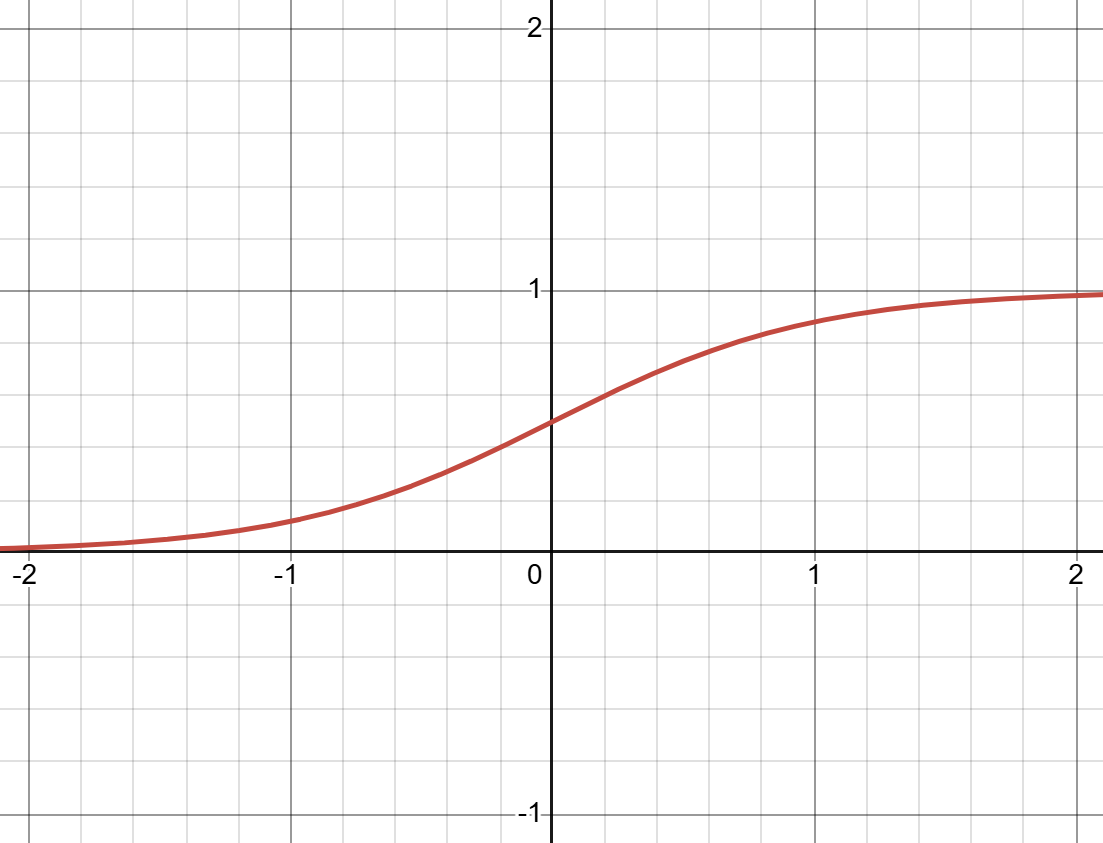
(H.Y. using Desmos)
Equation: \(\sigma(x)=\frac{1}{1+e^{-x}}\) activation, we would write that \(a^{(3)}=\sigma(z^{(3)})\). **. Similar to the previous bits of notation, we can also reference individual nodes using subscript indexing like \(\sigma(z_i^{(l)})\). - Now the weighted sum, otherwise known as the "linear combination", \(z^{(l)}\) is itself composed of the previous nodes multiplied by some weights
with an added bias term. All of the weights between layers \((l-1)\) and \(l\) are represented as \(W^{(l)}\), while the individual weight can be
found by using 2 indices (\(i\) for the input neuron and \(j\) for the output neuron) as such: \(w_{ji}^{(l)}\) (Why not \(ij\)? This will be explained
very shortly, but its basically to make our lives easier when doing some of the maths.). It is important to remember that while \(x\) and \(a^{(l)}\)
are vectors (1D arrays of numbers), \(W^{(l)}\) is a matrix
\[W^{(l)} = \begin{bmatrix}
w_{11}^{(l)} & w_{12}^{(l)} & w_{13}^{(l)} & \cdots & w_{1n}^{(l)}\\
w_{21}^{(l)} & w_{22}^{(l)} & w_{23}^{(l)} & \cdots & w_{2n}^{(l)}\\
\vdots & \vdots & \vdots & \ddots & \vdots \\
w_{m1}^{(l)} & w_{m2}^{(l)} & w_{m3}^{(l)} & \cdots & w_{mn}^{(l)}
\end{bmatrix}\]
A matrix is a rectangular grid of numbers or variables. In the context of neural networks, we usually talk about 2D matrices that represent all the weights (and sometimes biases) between two layers. These matrices normally have \(m \times n\) shape where \(n\) is the input index and the number of columns, and \(m\) is the output index and the number of rows. (a 2D array of numbers).
Weight Matrix Diagram (H.Y. using Canva and Overleaf)
Therefore, we write \(z^{(l)}=W^{(l)} a^{(l-1)} + b^{(l)}\), or \(z_{j}^{(l)}=w_{j1}^{(l)}a_1^{(l-1)}+w_{j2}^{(l)}a_2^{(l-1)}+\cdots+w_{jn}^{(l)}a_n^{(l-1)}+b_j^{(l)}\).
This equivalence is made possible by the very specific way that matrix / vector multiplication works.
Say for example we had the first hidden layer with 4 nodes, and the second with 3. Then we would write: \[a^{(2)}=f(Wa^{(1)}+b^{(2)})\] \[=f\left(\begin{bmatrix} w_{11}^{(2)} & w_{12}^{(2)} & w_{13}^{(2)} & w_{14}^{(2)}\\ w_{21}^{(2)} & w_{22}^{(2)} & w_{23}^{(2)} & w_{24}^{(2)}\\ w_{31}^{(2)} & w_{32}^{(2)} & w_{33}^{(2)} & w_{34}^{(2)} \end{bmatrix}\begin{pmatrix}a_{1}^{(1)} \\ a_{2}^{(1)} \\ a_{3}^{(1)} \\ a_{4}^{(1)}\end{pmatrix}+ \begin{pmatrix}b_{1}^{(2)} \\ b_{2}^{(2)} \\ b_{3}^{(2)}\end{pmatrix}\right)\] \[a^{(2)}=f\left(\begin{bmatrix} w_{11}^{(2)}a_{1}^{(1)} + w_{12}^{(2)}a_{2}^{(1)} + w_{13}^{(2)}a_{3}^{(1)} + w_{14}^{(2)}a_{4}^{(1)}\\ w_{21}^{(2)}a_{1}^{(1)} + w_{22}^{(2)}a_{2}^{(1)} + w_{23}^{(2)}a_{3}^{(1)} + w_{24}^{(2)}a_{4}^{(1)}\\ w_{31}^{(2)}a_{1}^{(1)} + w_{32}^{(2)}a_{2}^{(1)} + w_{33}^{(2)}a_{3}^{(1)} + w_{34}^{(2)}a_{4}^{(1)} \end{bmatrix} + \begin{pmatrix}b_{1}^{(2)} \\ b_{2}^{(2)} \\ b_{3}^{(2)}\end{pmatrix}\right)\]
Notice here how this only works if we index our nodes with the output index first and input second.
▬▬▬▬▬▬
Now that we have the mathematical tools to tackle MLPs, we can begin by writing out the formula for the output of a single neuron in our huge network:
\[a_j^{(l)}=f(w_{j1}^{(l)}a_1^{(l-1)}+w_{j2}^{(l)}a_2^{(l-1)}+\cdots+w_{jn}^{(l)}a_n^{(l-1)}+b_j^{(l)})\]
Or, using summation notation,
\[a_j^{(l)}=f\left(b_j^{(l)}+\sum_{i=1}^n w_{ji}^{(l)}a_i^{(l-1)}\right)\]
- Calculate the values of all of the weights \(w_{ji}^{(l)}\) multiplied by their corresponding neurons \(a_i^{(l-1)}\) in the previous layer.
- Sum up all of these values.
- Add to this the bias term \(b_j^{(l)}\).
- Put all of this through the activation function \(f\).
- Set the node \(a_j^{(l)}\) to this result.
where \(n\) is the number of neurons in the previous layer.
Then, we can expand this to an entire layer in our neural network:
\[a^{(l)}=f(W^{(l)}a^{(l-1)}+b^{(l)})\]
Now, for our multilayer perceptron, we simply combine many of these single layer equations together:
\[a^{(1)}=f(W^{(1)}x+b^{(1)})\]
\[a^{(2)}=f(W^{(2)}a^{(1)}+b^{(2)})\]
\[\vdots\]
\[a^{(L)}=f(W^{(L-1)}a^{(L-2)}+b^{(L-1)})\]
\[\hat{y}=f(W^{(L)}a^{(L-1)}+b^{(L)})\]
where \(\hat{y}\) is the model's output or prediction, and \(L\) is the number of layers in the neural network (excluding the input neurons, since they don't do anything except hold data).
▬▬▬▬▬▬
We have now defined something called forward propagation, which is the process where our inputs go through this complex web of calculations to reach the output. This is one of the most important, if not the most important process in neural networks. I the next tutorial, we will try to discover how our neural networks learns to make "good" predictions, the process of gradient descent and backpropagation.
Footnote on Activation Functions:
(H.Y. using Desmos)
A linear function, when graphed, produces a straight line. One of the most important features of linear functions is that they always have the same gradient or "derivative"., we would want to use a threshold function like Rosenblatt's step function, while tasks like image recognition benefit more from the non-linear sigmoid
(H.Y. using Desmos)
Equation: \(\sigma(x)=\frac{1}{1+e^{-x}}\) function. Other examples of activation functions include ReLU (Rectified Linear Unit)
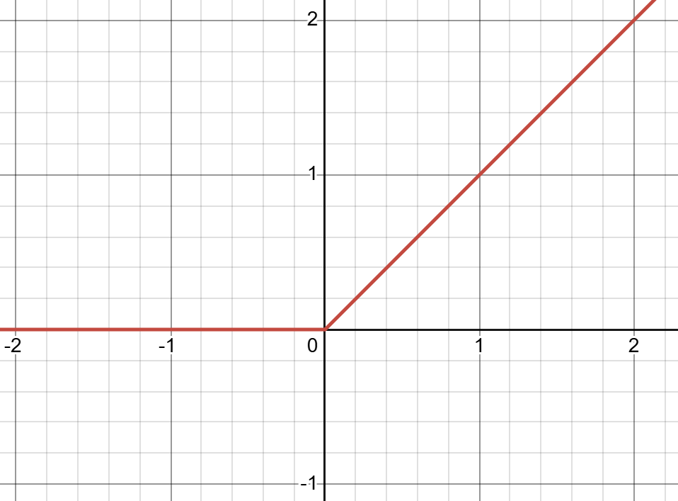
(H.Y. using Desmos)
Equation: \(f(x)=\begin{cases}0 \text{ if } x \leq 0 \\ x \text{ if } x > 0 \end{cases}\) and \(tanh\) (hyperbolic tangent)
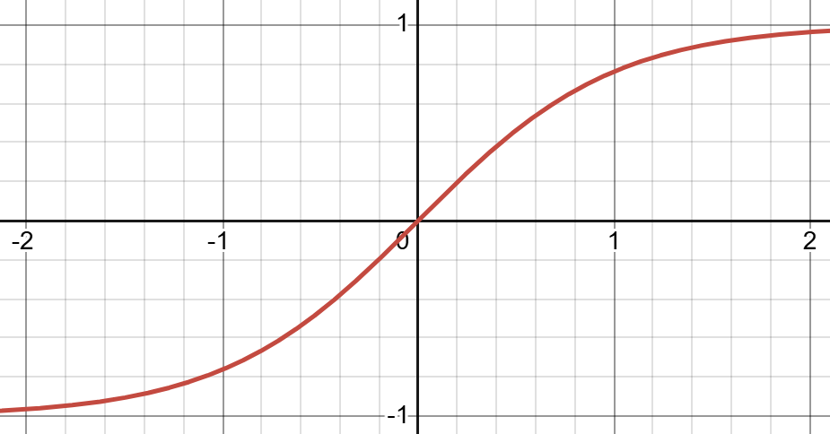
(H.Y. using Desmos)
Equation: \(f(x)=tanh(x)\). ↩